The Data Viewfinder

Reinforcement Learning (RL) is a subfield of machine learning where an agent learns how to make decisions by interacting with an environment. The agent’s goal is to learn a strategy, or policy, that maximizes some notion of cumulative reward over time.
Unlike supervised learning, where the model is trained on a fixed dataset, reinforcement learning is more dynamic: the agent learns from trial and error, receiving feedback in the form of rewards or penalties. This feedback loop allows the agent to improve its behavior gradually.

Understanding Q-Learning

Q-Learning is one of the simplest and most popular algorithms in reinforcement learning. It is a model-free method, meaning it does not require a model of the environment (i.e., no need to know transition probabilities). Instead, it learns a Q-function, which estimates the expected utility of taking an action in a given state and following the optimal policy thereafter.
The Q-value update rule is given by the Bellman equation:

Q(s,a) = Q(s,a) + α·(r + γ·max_a’ Q(s’,a’) – Q(s,a))

Where:

• s is the current state
• a is the action taken
• r is the reward received
• s’ is the resulting state
• α is the learning rate
• γ is the discount factor

Key Parameters

The learning rate determines how quickly the Q-values are updated. A higher learning rate means the agent prioritizes new information more, which can lead to faster learning but also more instability. A lower learning rate leads to slower, more stable learning.
The discount factor controls how much the agent values future rewards. A discount factor close to 0 makes the agent short-sighted, while a value close to 1 makes it strive for long-term rewards.
The exploration rate defines how often the agent takes a random action instead of the best-known one. This is essential to ensure that the agent explores the environment and doesn’t get stuck in suboptimal paths. Over time, is usually decayed to favor exploitation.

A Simple Example: 4 States, 2 Actions

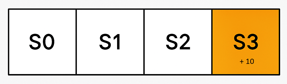
Let’s illustrate Q-learning with a minimal example. Consider an environment with 4 states in a straight line: S0, S1, S2, S3. The agent starts at S0, and the goal is to reach S3, which gives a reward of +10. All other actions give zero reward.

Available actions:

• ‘R’: move right (to next state)
• ‘L’: move left (to previous state)

The transition rules are deterministic. For instance, from S2, taking action ‘R’ moves to S3 and gives reward 10.

We initialize the Q-table with zeros. Initially, the table looks like this:

State	L (left)	R (right)
S0	0.0	0.0
S1	0.0	0.0
S2	0.0	0.0
S3	0.0	0.0

Now, we run two episodes with the following parameters:

• α = 0.5
• γ = 0.9
• ε = 0.0 ((purely greedy policy for simplicity)

Episode 1

1. Start at S0. All Q-values are 0. Agent chooses ‘R’.
2. Move to S1. Reward = 0. Update: no change in Q(S0, R).
3. At S1, choose ‘R’. Move to S2. Reward = 0. Update: no change in Q(S1, R).
4. At S2, choose ‘R’. Move to S3. Reward = 10. Update: Q(S2, R) = 0 + 0.5·(10 + 0.9·0 – 0) = 5.0

State	L (left)	R (right)
S0	0.0	0.0
S1	0.0	0.0
S2	0.0	5.0
S3	0.0	0.0

Episode 2

1. Start at S0. Choose ‘R’ again. Move to S1. Update: still zero.
2. At S1, choose ‘R’. Move to S2. Now Q(S2, R) = 5.0. Update Q(S1,R) = 0 + 0.5·(0 + 0.9·5.0 – 0) = 2.25
3. t S2, choose ‘R’. Move to S3. Update: Q(S2,R) = 5.0 + 0.5·(10 + 0 – 5.0) = 7.5

State	L (left)	R (right)
S0	0.0	0.0
S1	0.0	2.25
S2	0.0	7.5
S3	0.0	0.0

These results make it clear that the algorithm figures out the best thing to do is just keep moving to the right.

Because in this case we are using a greedy policy (the exploration rate is zero), the agent always selects the action with the highest Q-value.

On Convergence

Convergence in Q-learning means that the Q-values stabilize and stop changing significantly with further training. This typically happens when:

• The agent has explored all relevant state-action pairs.
• The learning rate decays (or is small).
• Sufficient episodes are run.

In our simple example, the Q-value for S2 → R should converge toward 10 (the immediate reward), and S1 → R should converge toward γ·10 = 9.0 . With more episodes, the Q-values will reflect the true expected return of each action.
Q-learning is a powerful but intuitive algorithm that demonstrates the core ideas of reinforcement learning: learning by interaction, trial and error, and maximizing cumulative reward.