The Data Viewfinder

Classification tasks are fundamental to machine learning because they address a wide range of real-world problems where the goal is to assign categories or labels to data points. From detecting spam in emails, recognizing handwritten digits, diagnosing diseases from medical images, to identifying fraudulent transactions—many practical applications rely on the ability to correctly classify inputs into discrete classes.

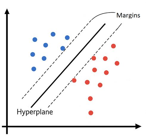
Support Vector Machines (SVMs) are powerful supervised learning algorithms used primarily for classification tasks. Their main goal is to find the optimal hyperplane that separates data points of different classes with the maximum margin—that is, the largest possible distance between the boundary and the closest data points from each class (called support vectors). Imagine you have two different objects, represented by blue and red. The points closest to the other group will have vectors associated with them—these are called support vectors. On top of those vectors, two parallel lines can be drawn; they are called margins. In the middle of the space defined by the margins lies the hyperplane, which is the central decision boundary that separates the classes.

Mathematically:

The hyperplane is represented by the following equation:

w ∙ x + b = 0 → w₁x₁ + w₂x₂ + b =0

Where:

• w = [w₁, w₂, …, w_n] is the weight vector, which controls the direction and slope of the boundary
• b is the bias (intercept) term
• x is the input feature vector

Our goal is to find w and b, such that:

• Points from class -1 satisfy: w ∙ x_i + b ≤ -1
• Points from class +1 satisfy: w ∙ x_i + b ≥ +1

Geometrically the weight vector is perpendicular to the hyperplane, and its magnitude, ||w||, is used to calculate the margin, which must be maximized

Margin = 2/||w||

Remember that maximizing 2/||w|| is the same as minimizing w, or w²/2

Now let’s consider we are working with a 4-points classification problem:

• Class +1: (2,2),(4,4)
• Class -1: (4,0),(6,2)

Solving the equations shown above for that set of points would lead to:

w = [1,1] and b = -4

So the hyperplane would be: x₁ + x₂ – 4 = 0

The margins (the lines that ‘touch’ the support vector) would be:

x₁ + x₂ -4 = 1 → x₁ + x₂ = 5

x₁ + x₂ -4 = -1 → x₁ + x₂ -4 = 3

And the margin width would be 2/||w|| = 2/(√(1²+1²) = 2/√2 = √2

This can be represented graphically as:

What if the data is not linearly separable?

When the data is not linearly separable at all (e.g., data in concentric circles), we transform it into a higher-dimensional space where a linear separator can be found.

Imagine trying to separate these 2D points:

• Class A: inside a circle
• Class B: outside the circle

A linear boundary won’t work in 2D, but it will if you map the points into a higher dimension using:

ϕ(x) = ϕ(x₁,x₂) = (x₁² + √(2x₁x₂) + x₂²)

Where x₁ and x₂ are features of the vector x.

Instead of doing this explicitly, SVM uses the kernel trick, which is a technique that allows the algorithm to learn non-linear boundaries without explicitly transforming the data (which would be extremally computationally expensive, since we would be adding new features). The trick here is to use the dot product between data points, so there is never an actual need to feature mapping function ϕ(x). The dot product is an operation between two vectors that produces a scalar number.

Considering the aforementioned mapping function, the dot product would be:

Φ(x)^T ϕ(x’) = (x₁x₁’)² + 2(x₁x₂) (x₁’x₂’) + (x₂x₂’)² = (x^T∙x’)²

This means we can define the polynomial kernel as K(x, x’) = (x^Tx’)², no need to compute the feature map Φ!

Here are some common Kernel Functions:

Kernel	Formula	Description
Linear	K(x, x’) = xTx’	No transformation
Polynomial	K(x, x’) = (xTx’+ c)d	Expands feature space with polynomial terms
RBF (Gaussian)	K(x, x’) = exp(-γ|| x – x’||2)	Infinite-dimensional! Smooth, localized boundaries
Sigmoid	K(x, x’) = tanh(κxTx’ + c)	Similar to neural network activations

In summary

Support Vector Machines (SVMs) are powerful for classification tasks, especially in high-dimensional spaces and when the number of samples is limited. They work well with clear margin separation and are effective with kernel functions for non-linear problems. However, SVMs can be computationally intensive with large datasets, sensitive to the choice of kernel and parameters, and less effective when data is noisy or overlapping.