
Oftentimes, when we compare two versions of a product, it’s difficult to tell whether the changes made in the alternative version are actually producing the expected results or if the differences we see could simply be due to chance. This is where statistical significance comes in; it represents the idea of measuring how likely it is that an outcome was caused by randomness rather than by a real change. In scientific literature, the term “statistically significant” appears frequently, and it refers to a result that is unlikely to have occurred by chance. In other words, it indicates that a particular treatment or change had a real, measurable impact on the results.
But how can we make sure a result is statistically significant? We can use a simple hypothesis test to answer that question. We begin with a straightforward assumption: that the result happened by chance, meaning our treatment or product change had no real impact. This is what we call the null hypothesis. In an A/B test, the null hypothesis states that both versions produce the same outcomes.
To test that hypothesis, we calculate the p-value, a statistical measure that indicates how probable it is that the difference in results came from chance alone. In other words, assuming both samples truly behave the same, the p-value represents the likelihood that the observed differences can be explained by random sampling.
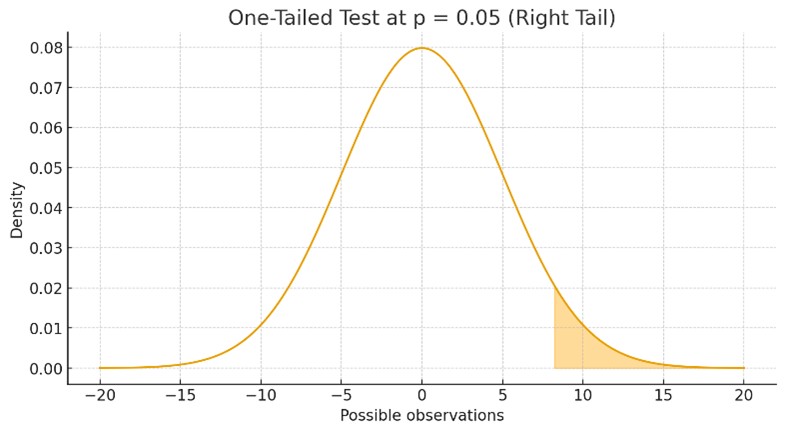
After calculating the p-value of our experiment, we compare it against a threshold, usually 0.05. A p-value of 0.05 means there is a 5% chance of observing results this extreme even if the null hypothesis is actually true. In other words, even when there is no real difference between the treatments, we would still expect to see results like these about 5% of the time purely by chance. By choosing 0.05 as our threshold, we are accepting a 5% false positive rate, a 5-in-100 chance of concluding that a change or treatment was effective when it actually was not. When talking about hypothesis tests, there are two ways to evaluate an alternative hypothesis. We can test whether version B is simply different from version A (a two-tailed test) or whether version B is specifically better or worse than A (a one-tailed test). The difference between these approaches becomes much easier to see when looking at the graphics below

To calculate a p-value we need to choose the appropriate statistical test, since each test defines how we measure the probability of observing our results by chance. In A/B testing with discrete variables, this typically means selecting a test that matches the structure of the data: proportion z-tests, chi-square tests, and Fisher’s exact test for binary outcomes, or Poisson-based tests for count data. Each method uses the same core idea, but the mathematical form of the p-value depends on the assumptions behind the test.
Fisher’s Exact Test
Fisher’s Exact Test becomes especially useful when we are working with small sample sizes, where the common approximations used in other tests (like the z-test or chi-square test) may no longer be reliable. Instead of relying on a normal approximation, Fisher’s method computes the exact probability of observing a table of outcomes as extreme as the one in our experiment, assuming there is no real difference between the groups. This makes it a robust choice for low-traffic A/B tests or early experiments where only a small number of users have been exposed to each version.
Proportion z-test
The proportion z-test is the standard approach for analyzing binary metrics in large-sample A/B tests. It relies on the idea that, with enough observations, the difference between two proportions (such as CTR, conversion rate, or bounce rate) follows a normal distribution. This allows us to estimate how far apart the two versions are in standardized units and then calculate a p-value. Because it works well with high traffic and binary outcomes, it is one of the most widely used tests in product experimentation.
Chi-square test
The chi-square test and the proportion z-test are closely related, and in many A/B testing scenarios they lead to almost identical conclusions. Both are used to analyze binary outcomes, such as click-through rate or conversion rate, and both aim to determine whether the difference between two groups is larger than what we would expect by chance. The main difference lies in how they approach the problem. The z-test compares proportions directly and assumes the sampling distribution of that difference is approximately normal when sample sizes are large. The chi-square test, on the other hand, works with counts in a contingency table and measures how far the observed frequencies deviate from the frequencies we would expect if both groups behaved the same.
When to use each test
In practice, the proportion z-test is often preferred for A/B tests because it is specifically designed for comparing two proportions and is straightforward to interpret. The chi-square test becomes useful when the results are naturally presented in a contingency table or when comparing more than two groups or more than two categorical outcomes. However, the chi-square test still relies on large expected counts, so it should not be used when sample sizes are small. In low-traffic experiments, Fisher’s Exact Test is the appropriate alternative.
If you are comparing two proportions with a reasonably large sample size, the z-test is typically the simplest and most direct choice. The chi-square test becomes a flexible complement when your data structure or experimental design involves categorical outcomes beyond a simple binary comparison.
Testing a New Layout: A Practical Example Using Synthetic Data
Imagine we were hired by an e-commerce company that wants to test a new layout for their website, featuring a clearer call-to-action button (in this case, “Purchase”). Our scenario looks like this:
- Variant A (control): current layout
- Variant B (treatment): new layout with clearer call-to-action button
To evaluate whether the new layout encourages users to purchase more, we focus on the following metrics:
- Click-Through Rate (CTR): clicks on ‘Purchase’ divided by total visitors
- Conversion Rate: purchases divided by total visitors
Both metrics represent user actions and will be encoded as 0 when the visitor did not take the action and 1 when they did. The dataset we will use contains 5,000 entries with four columns: user_id, group (control or treatment), clicked (0/1), and converted (0/1).
(The dataset we are using is synthetic and serves only to demonstrate how to perform the test.)
Below the propabilities of success for each metric and group are given:
| CTR | Conversion Rate | |
| Control | 0.1492 | 0.0404 |
| Treatment | 0.1796 | 0.0388 |
Calculating the z-score
The z-test relies on the fact that, with a large enough sample, the difference between two proportions follows a normal distribution. This allows us to convert that difference into a z-score and use the properties of the normal curve to determine how extreme our result is and calculate the corresponding p-value.
The probability of a user, part of the control group, clicking on the Purchase button is 0.1492. For the Treatment group is 0.1796. If we calculate the standard error considering all the participants of both groups, we can calculate the z-score as (0,1796 – 0,1492)/(standard error). Mathematically:
For our hypothesis of CTR being different in the control and treatment groups, the calculated z-score was -2.9.
Calculating and understanding the p-value
To understand what exaclty is the p-value and how it is obtained let’s start by plotting a normal distribution.

Looking at this distribution, we can interpret the probability of a value being smaller than a given z-score as the area underneath the curve. For example, if the z-score is 0, there is a 50% chance of a value being smaller than that. This probability is given by the CDF (Cumulative Distribution Function). The p-value for a two-tailed test is calculated as 2 × (1 − CDF(|z|)). For instance, imagine the z-score is −2. In that case, CDF(|−2|) represents the entire area from −∞ to +2 (because we use the absolute value). The expression (1 − CDF(|z|)) gives the area above z = 2, which is equal to the area below z = −2, since the normal curve is symmetric. Because this is a two-tailed test, meaning we are checking for any difference between the groups, this tail probability is multiplied by 2.
Two-tailed p-value
Right-tailed p-value
Left-tailed p-value
For this case the calculated two-tailed p-value was 0.0037
In Python both the z-score and the p-value can also be computed automatically using the statsmodels library, which provides built-in functions for two-sample proportion tests.
The obtained p-value (0.0037) is well below the commonly used 0.05 threshold, so we reject the null hypothesis and conclude that the control and treatment groups show statistically different results. This can be seen clearly in the graphic below:
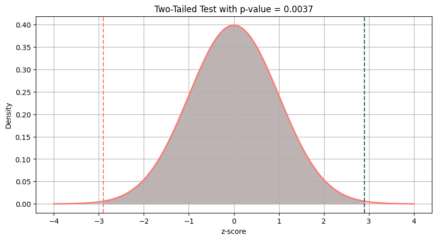
The total area in the shaded tails (above and below the vertical lines) represents the probability of observing a result at least this extreme if the null hypothesis is true. From the figure, we can already see that this probability is very close to zero.
Conversion Rate
Now that we’ve analyzed the CTR, we can do the same for the conversion rate. But instead of using a two-tailed test, we will run a left-tailed test. Since the conversion rate of B was smaller (as shown in our table), we will test the hypothesis that B performs worse than A.
After running the calculations, we obtained a p-value of 0.39. This value is far too large to reject the null hypothesis, meaning that the observed difference in conversion rates is well within what we would expect from random variation.
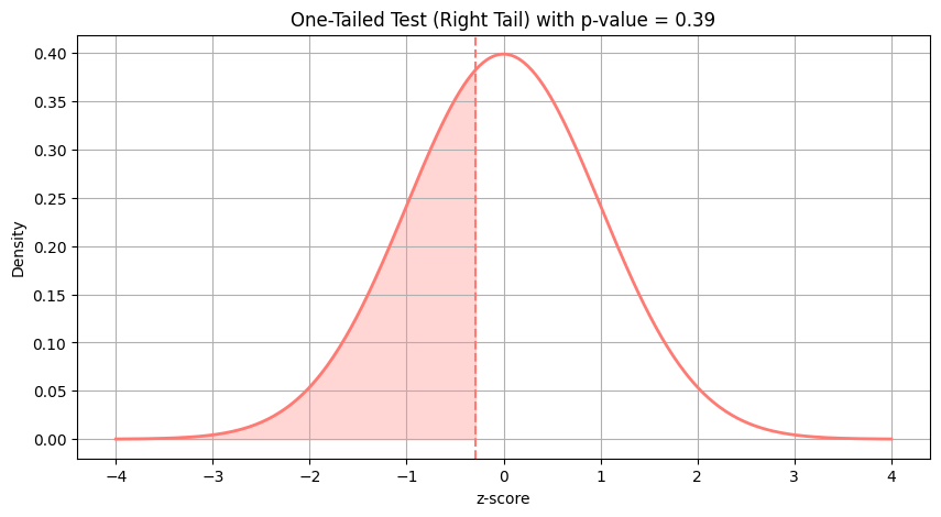
The shaded area represents the probability of obtaining a result where B appears smaller than A purely by chance, assuming the null hypothesis is true and both groups have the same underlying conversion rate. Because this probability is quite high, we do not have evidence to reject the null hypothesis, meaning the conversion rate did not increase after changing the layout.
Visual Reports
CTR and Conversion Rate by Group
This chart shows the average CTR and conversion rate for each group. While the variant clearly improved CTR, the conversion rates remain nearly identical, suggesting that increased engagement did not translate into more purchases.

Funnel Comparison
The funnel chart visualizes the flow from visitors to clicks to conversions. The variant generates more clicks, but both funnels narrow to almost the same point at the final step, reinforcing that conversions did not meaningfully increase.

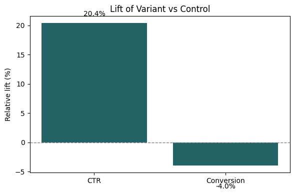
Lift of Variant vs. Control
The lift chart highlights the relative impact of the new layout. We see a positive lift for CTR but almost no lift for conversion, further illustrating that the layout change influenced user behavior at the top of the funnel but not at the final decision stage.
Conclusion
Taken together, these analyses show that the new layout successfully encouraged more users to engage with the page but did not lead to more purchases. In other words, the design improved CTR but did not impact the overall conversion rate. This highlights the importance of evaluating multiple metrics in A/B tests, as changes that increase engagement do not always translate into meaningful business outcomes.

Leave a comment